Some Advanced Methods for Volatility estimation
When we calculate volatility using the customary methods we don't take into account the order of observations. Additionally, all observations have equal weights in the formulas. But the most recent data about asset's return movements is more important for volatility forecasting than more dated data. That is why, the recently recorded statistical data should be given more weight for forecasting purposes than older data. One of the models that operate off of this assumption is the exponentially weighted moving average.
Simple Moving Average (SMA)
The Moving Average is an average of a set of variables such as stock prices over time. The term "moving" steams from the fact that as each new price is added, the oldest price is subsequently deleted. The n-day Simple Moving Average takes the sum of the last n days prices. The SMA model is probably the most widely used volatility model in Value at Risk studies.
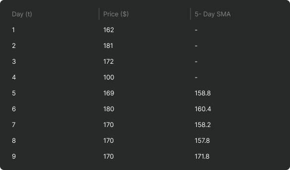
The disadvantage of the SMA is that it is inherently a memory-less function. A major drop or rise in the price is forgotten and does not manifest itself quantitatively in the simple moving average. As you can see in the following table, on day 9 there is a big step in the simple moving average, while price has been constant at $170. This distortion is caused by the low price on day 4 - dropped from the SMA on day 9.
Exponentially Weighted Moving Average (EWMA)
This section discusses the J.P. Morgan RiskMetrics? approach to estimating and forecasting volatility that uses an exponentially weighted moving average model (EWMA).
The EWMA model allows one to calculate a value for a given time on the basis of the previous day's value. The EWMA model has an advantage in comparison with SMA, because the EWMA has a memory. The EWMA remembers a fraction of its past by a factor A, that makes the EWMA a good indicator of the history of the price movement if a wise choice of the term is made. Using the exponential moving average of historical observations allows one to capture the dynamic features of volatility. The model uses the latest observations with the highest weights in the volatility estimate.
Initial value of volatility is taken as standard deviation of recent N returns (r1, r2, ..., rN ) of N+1 days.
\(\sigma_{1}^{2} = \frac{1}{N - 1} \displaystyle\sum_{t=2}^{N + 1} \lparen r_{t} - \bar{R} \rparen^{2} \)
Expected volatilities \(\sigma_{2}, \sigma_{3}, \sigma_{4}, ... \) in the EWMA model are calculated by the following formula:
\(\sigma_{n}^{2} = \lambda * \sigma_{n - 1}^{2} + \lparen 1 - \lambda \rparen * \gamma_{n - 1}^{2} \)
\( \sigma_{n}^{2} \) - a dispersion estimate for the day n calculated at the end of the (n - 1) day.
\( \sigma_{n - 1}^{2} \) - a dispersion estimate for the day (n-1).
\( \gamma_{n - 1} \) - asset's return for the day (n - 1). Return for the day n is calculated as the natural logarithm of the ration of a stock's price from the day n to previous day n - 1
\( \lambda \) - decay factor.
The exponentially weighted moving average model depends on the parameter \( \lambda \lgroup 0 < \lambda < 1 \rgroup \) which is often referred to as the decay factor.
Firstly, this parameter defines a relative weight \( \lgroup 1 - \lambda \rgroup \) , that is applied to the last return.This weight also defines the effective amount of data used in estimating volatility. The more the \( \lambda \) value, the less last observation affects the current dispersion estimation. Secondly, defines the rate of dispersion return to the previous level. The greater the value, the faster dispersion will come back to the previous level after strong return change. The optimal value for current daily dispersion (volatility) is \( \lambda \) = 0.94
For such a value, the evaluation of dispersion can be done on the basis of 50 observations, and return of first day (r1) will be considered with the relative weight of (1-0.94)*0.94^49=0.0029. Even for 30 observations the error will be insignificant.
The formula of the EWMA model can be rearranged to the following form:
\(\sigma_{1}^{2} = \lgroup 1 - \lambda \rgroup \displaystyle\sum_{t=1}^{\infty} \lambda^{-1} * \gamma_{n - T}^{2} \)
Thus, the older returns have the lower weights, which are close to zero.
Note, in the standard formula we take all returns with the same weight 1/(N-1)
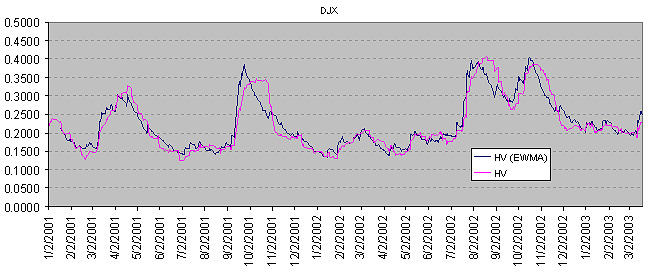
The chart below shows 30 day historical volatility calculated by the EWMA method and the ordinary historical volatility calculated as a standard deviation of stock returns. As you can see EWMA Volatility almost agrees with ordinary historical volatility, but advantage of using EWMA is that this model requires only the last day's data and no additional recalculations.
The high low historical volatility also can be calculated by the EWMA method. In this case return rt must be calculated as the natural logarithm of the ratio of a stock's high price from the day n to stock's low price from the day t.
And the initial volatility value \(\sigma_{1}\) is taken as Parkinson's number for the recent N days.