Logarithmic Garman Klass (LGK)

\(\gamma_{t}^{2} = (\ln \frac{O_{t}}{C_{t-1}})^{2} + 0.5*(\ln \frac{H_{t}}{L_t})^{2} - 0.39*(\ln \frac{C_{t}}{O_{t}})^{2} \)

where \(\gamma_{t}^{2} \) is volatility metric ( \( \gamma_{2}^{2} , \gamma_{3}^{2} \) ?)

Ot, Ht, Lt, Ct are respectively, open, high, low, and close price for the day t. Thus the volatility metric is a combination of the overnight, high/low and open/close range. Such a volatility metric is a more efficient measure of the degree of volatility during a given day. This metric is always positive. Thus, expected volatility can be calculated from the following recurrent formula

\(\ln(\sigma_{t}^{2} ) = ( 1 - \lambda ) * \ln(\gamma_{t-1}^{2}) + \lambda * \ln(\sigma_{t - 1}^{2})\)

The advantage of the logarithmic transform is that the residuals in the forecasting equation are approximately normal.

Expected volatility is

\( \sigma_{t} = \sqrt{\exp\left((1 - \lambda) * \ln(\gamma_{t - 1}^{2}) + \lambda * \ln(\sigma_{t - 1}^{2})\right)} \)

The parameter \( \lambda \) can be taken equal to 0.9049.

Initial value \( \sigma_{2} \) is taken as:

\( \sigma^2 = \frac{\displaystyle\sum_{i=2}^{N+1} (\gamma_i - \bar{\gamma})^2}{N - 1} \) where \( \bar{\gamma} \) - is the mean of close-to-close

returns: \( \bar{\gamma} = \frac{\displaystyle\sum_{2}^{N+1} \ln \frac{C_t}{C_{t-1}}}{N} \)

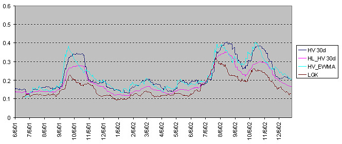
The following chart shows ordinary historical volatility (calculated as standard deviation of stock's returns), High Low Historical Volatility, volatility calculated by the EWMA method on the basis of the initial volatility taken as a standard deviation, and volatility calculated by using the LGK model.